Predictive Habitat models - GRASS and R-stats
[ updated 10/2005 to GRASS 6, we recommend 6.1 ]
GIS Application: Simple predictive model for presence of beetles
Introduction
In this section we want to generate a beetle (bugs) presence prediction map
in the Spearfish (SD, USA) region based on vegetation, elevation and other variables.
Data: Given is a map with observed beetles presence ('bugsites' map in Spearfish
data set). Additionally we have several maps describing elevation, vegetation, geology, etc.
Concept: For every spot with observed beetles presence (by coordinates) we will
select further variables. This will give us an idea where und under which environmental
conditions beetles may be present in the study area. To enhance the number of variables,
we will use GIS functionality to additional generate (derived) variables such as
distance to water etc.
To create a predictive model we also need beetles absence data including the environmental
conditions. Unfortunately there are no observed absence data in our data set; thus we have
to construct synthetically absence data. Using the (over)simplified assumption that beetles
are absent where no beetles were observed, we can extract these variables from the maps.
In GIS, we can select sites where beetles are absent by masking the buffered presence sites.
As before, we also extract further environmental variables for the absence sites.
Both presence and absence data including the environmental conditions we finally write
into a table:
            +------------> Beetle site (with related data: | veg | elev | geology | etc)
     +------|---+               P: presence, A: absence
    /  veg  *  /
   /          /-+
  +----------+ /           x | y | elev|Beetle| veg    | geol| ...
   /   elev   /-+         ---+---+-----+------+--------+-----+-----
  +----------+ /           ..| ..| 1200|  P   | wood   | cl. | ...
   /   geol   /-+          ..| ..| 1432|  P   | wood   | s.  | ...
  +----------+ /           ..| ..|  345|  A   | pasture| ft. | ...
   /    ...   /            [...]
  +----------+
Note that it is more conventient to create this table in GRASS instead of R
because reading numerous large raster maps into R requires a lot of memory
(there is a sample() function in R, though).
Prediction: We read this table into R and run a predictive model on the data
(here: using 'rpart'). The resulting tree, after pruning and optimizing it, we use for the
prediction. The prediction itself is done on the full GRASS maps read into R. It's important
to create an index of "no data" (NA) cells to prevent predictions for these cells. Finally
we write out the prediction map as well as beetles presence/absence probability maps back
to GRASS.
First start GRASS with Spearfish 6 data set:
grass60
# select: LOCATION: spearfish60
#         MAPSET: create a new mapset with your login name

#set region, set resolution (we lower here the resolution to avoid
# heavy computations - please keep it high (10m) at home):
g.region rast=elevation.10m res=30 -p

#fetch info about beetles (bugs) observations vector points map (this
#map is stored in the PERMANENT mapset):
v.info bugsites

#display column types and names in attribute table:
v.info -c bugsites

#check where the attribute table is stored (in which DBMS, usually DBF file):
v.db.connect -p bugsites

#look at the maps:
d.mon x0
d.rast elevation.10m
d.vect bugsites icon="basic/diamond" fcol=red
The spatial "ingredients" for the (simple) predictive modeling are:
- elevation map, slope, aspect;
- vegetation or landuse/landcover map derived from LANDSAT-7;
- geology;
- distance to water.
Extracting further environmental variables from maps
#calculate slope and aspect from elevation:
r.slope.aspect el=elevation.10m as=elev.as sl=elev.sl

#Preparation of distance-to-water map:
#we use the "streams" map from the data set
# (alternative: t_hydro vector streams map)
r.mapcalc "allarea.one=1"

# (option: use slower, but more accurate -k flag in r.cost)
r.cost in=allarea.one out=distance2water start_rast=streams percent=100
d.rast distance2water
r.info -r distance2water

#convert the pixel distances to meters:
r.mapcalc "dist2water.m=distance2water * (ewres() + nsres())/2.0"
r.info -r dist2water.m
g.remove distance2water
r.colors dist2water.m col=byr
d.rast dist2water.m

#we can overlay the distances-to-water map and the elevation model
#with semitransparency:
d.his h=dist2water.m i=elev.as
#also overlay the streams
d.rast -o streams
Updating the 'bugsites' attribute table
Now we have to extend the attribute table of the 'bugsites' vector
map. We want to add extra columns for storage of further environmental
variables. But we'll first check the database settings in our current
mapset and then copy the original 'bugsites' vector map into our own
mapset with a new name:
#check general DB settings for db.* commands in current mapset
# (these settings are handled individually for each mapset):
db.connect -p
#-> should be connected to DBF per default

#NOTE for "older" GRASS versions (fixed 18 Oct 2005):
           #if you are using GRASS before 6.0.2 or 6.1.x, you have to
           #execute the following two commands (fixed in later GRASS versions):

           db.connect driver=dbf database='$GISDBASE/$LOCATION_NAME/$MAPSET/dbf/'
           mkdir `g.gisenv GISDBASE`/`g.gisenv LOCATION_NAME`/`g.gisenv MAPSET`/dbf
           #

#We copy over the 'bugsites' map into our mapset with new name (...as you cannot
#work on a map in a different mapset - 'bugsites' is stored in PERMANENT:
g.copy vect=bugsites,mybugsites

#Now we add the new columns to the 'mybugsites ' map:
# - Add 'elevation' column, type DOUBLE
# - Add 'slope' column, type DOUBLE
# - Add 'aspect' column, type DOUBLE
# - Add 'vegetation' column, type INTEGER
# - Add 'geology' column, type INTEGER
# - Add 'dist2water' column, type DOUBLE

#In "older" GRASS 6.0.1, do:
           echo "ALTER TABLE mybugsites ADD COLUMN elevation double" |db.execute
           echo "ALTER TABLE mybugsites ADD COLUMN slope double" |db.execute
           echo "ALTER TABLE mybugsites ADD COLUMN aspect double" |db.execute
           echo "ALTER TABLE mybugsites ADD COLUMN vegetation integer" |db.execute
           echo "ALTER TABLE mybugsites ADD COLUMN geology integer" |db.execute
           echo "ALTER TABLE mybugsites ADD COLUMN dist2water double" |db.execute

#in GRASS 6.1.x, simply do:
v.db.addcol mybugsites col="elevation double,slope double,aspect double,vegetation integer,geology integer,dist2water double"

#verify:
v.info -c mybugsites
# -> the 'str1' column represents the presence of beetles (we use it later).
Now we have extended the 'mybugsites' table and can insert the
corresponding values of the environmental variables for each row
(equivalent to each beetle observation):
#read elevations at each bug site position and update the attribute table:
v.what.rast vect=mybugsites rast=elevation.10m col=elevation

#read slope at bug site positions and update the attribute table:
v.what.rast vect=mybugsites rast=elev.sl col=slope

#read aspect at bug site positions and update the attribute table:
v.what.rast vect=mybugsites rast=elev.as col=aspect

#read vegetation type at bug site positions and update the attribute table:
v.what.rast vect=mybugsites rast=vegcover col=vegetation

#read geology type at bug site positions and update the attribute table:
v.what.rast vect=mybugsites rast=geology col=geology

#read distance to water at bug site positions and update the attribute table:
v.what.rast vect=mybugsites rast=dist2water.m col=dist2water

#verification: check table contents:
echo "SELECT * FROM mybugsites" | db.select

#alternatively, you can simply use:
v.db.select mybugsites

#this also permits simple SQL queries:
v.db.select mybugsites where="elevation>1700"

#also enjoy interactive queries in the map:
d.vect mybugsites
d.what.vect

#to remember the vegcover and geology classes meanings, run:
r.report vegcover
r.report geology
Exporting beetles presence data set for R import
Since the GRASS/R interface is not yet updated to support vector data,
we export the 'mybugsites' map and the associated table to ASCII for
later import into R:
#Export of geometry (we use 'Unix piping/redirection' to store the output
#into a file instead of printing to the terminal) :
v.out.ascii mybugsites > mybugsites.coords
#verification of file (find in current directory):
nedit mybugsites.coords

#Export of attributes:
#  echo "SELECT cat,elevation,slope,aspect,vegetation,geology,dist2water,str1 FROM mybugsites" | db.select -c > mybugsites.atts
#easier to do in GRASS 6:
v.db.select -c mybugsites col="cat,elevation,slope,aspect,vegetation,geology,dist2water,str1" > mybugsites.atts

nedit mybugsites.atts
#- > that is the presence data set.
Preparing the beetles absence data set
Now we have to generate synthetic absence data (where we assume that beetles
aren't present). For this we buffer and mask out all beetles presence
sites, then we randomly sample absence from the remaining areas.
This is an oversimplification and may not be done in a real-life project!
Note: v.random doesn't help as it does not respect a raster MASK
(but: you could filter the result with a vector map and v.select).
#Generating absence data:
g.region rast=elevation.10m res=30 -p
v.to.rast in=mybugsites out=mybugsites use=cat
d.rast mybugsites
# the dots are nearly invisible... because of 10m resolution.

#use a 200m buffer around each bug site:
r.buffer in=mybugsites out=mybugsites.buf dist=200
r.mapcalc "MASK=if(isnull(mybugsites.buf),1,null())"
g.remove rast=mybugsites,mybugsites.buf

#verify MASK with elevation map, it should show holes:
d.rast elevation.10m

#how many bug sites do we have?
v.info mybugsites
# -> points: 90, so we want to generate 90 random points without bugs:

#generate random vector points stored in 'nobugs' map from the masked elevation map:
r.random in=elevation.10m n=90 vector_output=nobugs
d.vect nobugs
g.remove MASK

#let's look at the attribute table:
v.db.select nobugs

#...the table is already populated with the elevations of the absence points.
v.info -c nobugs

#NOTE: to later avoid column renaming, we add again a new column 'elevation'
#      and we'll ignore the 'value' column which already contains the elevation:

#In "older" GRASS 6.0.1, do:
           echo "ALTER TABLE nobugs ADD COLUMN elevation double" |db.execute
           echo "ALTER TABLE nobugs ADD COLUMN slope double" |db.execute
           echo "ALTER TABLE nobugs ADD COLUMN aspect double" |db.execute
           echo "ALTER TABLE nobugs ADD COLUMN vegetation integer" |db.execute
           echo "ALTER TABLE nobugs ADD COLUMN geology integer" |db.execute
           echo "ALTER TABLE nobugs ADD COLUMN dist2water double" |db.execute
           echo "ALTER TABLE nobugs ADD COLUMN str1 varchar(21)" |db.execute

#in GRASS 6.1.x, simply do:
v.db.addcol nobugs col="elevation double,slope double,aspect double,vegetation integer,geology integer,dist2water double,str1 varchar(21)"
v.info -c nobugs

#read elevations at nobug site positions and update the attribute table:
v.what.rast vect=nobugs rast=elevation.10m col=elevation

#read slope at nobug site positions and update the attribute table:
v.what.rast vect=nobugs rast=elev.sl col=slope

#read aspect at nobug site positions and update the attribute table:
v.what.rast vect=nobugs rast=elev.as col=aspect

#read vegetation type at nobug site positions and update the attribute table:
v.what.rast vect=nobugs rast=vegcover col=vegetation

#read geology type at nobug site positions and update the attribute table:
v.what.rast vect=nobugs rast=geology col=geology

#read distance to water at nobug site positions and update the attribute table:
v.what.rast vect=nobugs rast=dist2water.m col=dist2water

#Update the 'str1' column which will later be used as absence indicator with 'no beetles':
echo "UPDATE nobugs SET str1='no beetles' WHERE str1 is NULL" | db.execute

#verification:
echo "SELECT * FROM nobugs" | db.select

#or in GRASS 6, simply:
v.db.select nobugs
# -> should report a nice table

# AGAIN: this absence table will certainly contain potential beetles habitat
#        sites, remember that we use a very simple model here.

d.vect nobugs icon="basic/diamond" col=green
d.what.vect
Exporting beetles absence data set for R import
Since the GRASS/R interface is not yet updated to support vector data
[work is ongoing for the new GRASS 6/R interface, see "GRASS Newletter"],
we export the 'nobugs' map and the associated table to ASCII for later
import into R:
#Export of geometry:
v.out.ascii nobugs > nobugs.coords
nedit nobugs.coords

#Export of attributes:
# echo "select cat,elevation,slope,aspect,vegetation,geology,dist2water,str1 from nobugs" |db.select -c > nobugs.atts
#easier to do in GRASS 6:
v.db.select -c nobugs col="cat,elevation,slope,aspect,vegetation,geology,dist2water,str1" > nobugs.atts
nedit nobugs.atts
cat mybugsites.coords nobugs.coords > allsites.coords
wc -l allsites.coords
# 180 allsites.coords
nedit allsites.coords

cat mybugsites.atts nobugs.atts     > allsites.atts
wc -l allsites.atts
# 180 allsites.atts
nedit allsites.atts

#The polishing of this table we'll do later in R.
Starting the modeling session
At this point we have finished the data preparations.
Now we enter into R to generate the predictive map. Since the GRASS/R interface
completely changed for GRASS 6, we recommend to first read
GRASS News vol.3, June 2005
(R. Bivand. Interfacing GRASS 6 and R. GRASS Newsletter, 3:11-16, June 2005. ISSN 1614-8746).
Below examples are still reflecting the GRASS 5 interface and will be updated in
short time (Installation of R/GRASS6 interface: here):
R
#library(GRASS)
#G <- gmeta()

library(spgrass6)
# this will load some required packages...
G <- gmeta6()

#start the local help system in a Web browser (e.g., look at Packages -> 'spgrass6'):
help.start()

#import first table (coords):
mybugsites.coords <- read.table("allsites.coords", header=F, sep="|")
str(mybugsites.coords)
#... is a data.frame with 180 obs. of  3 variables.

#import second table (atts):
mybugsites.atts <- read.table("allsites.atts", header=F, sep="|")
str(mybugsites.atts)
#... is a data.frame with 180 obs. of  8 variables.

#bind together presence and absence data (but: don't merge tables by bug ID!):
mybugsites <- cbind(mybugsites.coords,mybugsites.atts)
names(mybugsites) <- c("east","north","id1","id2","elevation","slope",
                       "aspect","vegetation","geology","dist2water","presence")
mybugsites
str(mybugsites)
#... is now a data.frame with 180 obs. of 11 variables.

#we change the contents of the presence column to "P" for presence and "A" for absence:
#store it as factors (categorial data):
mybugsites$presence <- as.character(mybugsites$presence)
mybugsites$presence[mybugsites$presence=="no beetles"] <- "A"
mybugsites$presence[mybugsites$presence=="Beetle site"] <- "P"
mybugsites$presence <- as.factor(mybugsites$presence)
str(mybugsites)

#also change next variable types to factors:
mybugsites$vegetation <- as.factor(mybugsites$vegetation)
mybugsites$geology <- as.factor(mybugsites$geology)
str(mybugsites)
#... should report something like this (since we used random sampling, it varies):
#'data.frame':   180 obs. of  11 variables:
# $ east      : int  590232 590430 590529 590546 590612 590744 590810 590810 590843 590926 ...
# $ north     : int  4915039 4915204 4914625 4915353 4915320 4915535 4915303 4917635 4918544 4915518 ...
# $ id1       : int  1 2 3 4 5 6 7 8 9 10 ...
# $ id2       : int  1 2 3 4 5 6 7 8 9 10 ...
# $ elevation : num  1610 1611 1652 1671 1689 ...
# $ slope     : num  34.4 28.4 29.9 19.4 24.9 ...
# $ aspect    : num  133 290 214 277 237 ...
# $ vegetation: Factor w/ 6 levels "1","2","3","4",..: 3 3 3 3 3 2 3 3 3 3 ...
# $ geology   : Factor w/ 8 levels "1","3","4","5",..: 2 2 2 3 3 3 3 4 2 3 ...
# $ dist2water: num  60 360 180 180 180 0 210 0 690 30 ...
# $ presence  : Factor w/ 2 levels "A","P": 2 2 2 2 2 2 2 2 2 2 ...

#we can also summarize it:
summary(mybugsites)
R: graphical exploration of variables (beetles presence versus absence)
Now we can graphically check absence/presence occurency for the
various variables with box- and whiskerplots (we could also use the more powerful
bwplot() of the lattice library instead of boxplot() function).
Note: A boxplot displays if the data is symmetric or has suspected outliers.
A classical boxplot has a box with lines at the lower hinge (basically first quartile, Q1),
the median, the upper hinge (basically third quartile, Q3) and whiskers which extend to the
minimum and maximum.
The whiskers are shortened to a length of 1.5 times the box length (convention).
Any points beyond that are plotted with points to indicate outliers:
                       |  +---+-------+          |
                       |  |   |       |          |
       o oo o          +--+   |       +----------+    o  oo oo   o
                       |  |   |       |          |
                       |  +---+-------+          |

     [OutlierPoints]  Min Q1 Median   Q3        Max [OutlierPoints]
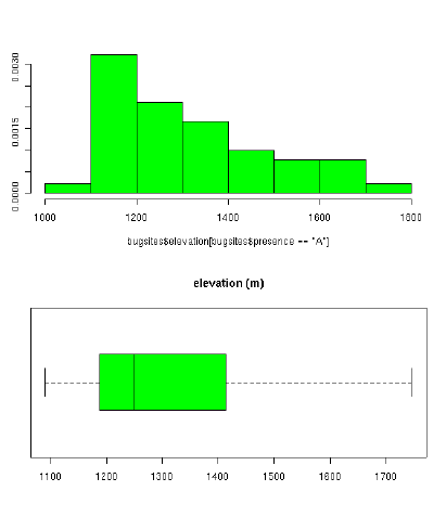
#Example to illustrate histogram and boxplot:
par(mfrow=c(2,1))
library(MASS)
truehist(mybugsites$elevation[mybugsites$presence=='A'], col="green")
  boxplot(elevation[presence=='A'] ~ presence[presence=='A'], data=mybugsites,
  col="green", main="elevation (m)", horizontal=TRUE)
par(mfrow=c(1,1))
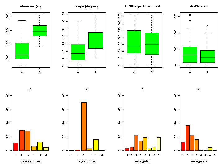
We continue with out sample data set:
#activate multiple graphs:
par(mfrow=c(2,4))

#show numerical data as boxplot:
boxplot(elevation ~ presence, data=mybugsites, col="green", main="elevation (m)")
boxplot(slope ~ presence, data=mybugsites,col="green", main="slope (degree)")
boxplot(aspect ~ presence, data=mybugsites,col="green", main="CCW aspect from East")
boxplot(dist2water ~ presence, data=mybugsites,col="green", main="dist2water")

#show factor data as boxplot:
barplot(summary(mybugsites$vegetation[mybugsites$presence=="A"]),
        ylim=c(0,80), xlab="vegetation class", main="A")
barplot(summary(mybugsites$vegetation[mybugsites$presence=="P"]),
        ylim=c(0,80), xlab="vegetation class", main="P")
barplot(summary(mybugsites$geology[mybugsites$presence=="A"]),
        ylim=c(0,80), xlab="geology class", main="A")
barplot(summary(mybugsites$geology[mybugsites$presence=="P"]),
        ylim=c(0,80), xlab="geology class", main="P")
par(mfrow=c(1,1))

#These plots can be used to understand the importance or usability of
#variables to predict presence/absence:


#Plotting data as map:
#just for plotting purpose we read in 'elevation.10m' and 'vegcover' map:
elev <- rast.get6("elevation.10m",cat=FALSE)
veg  <- rast.get6("vegcover",cat=TRUE)
str(elev)
str(veg)

#plot the bugs (beetles) presence on top of the 'elevation' map:
image(elev, "elevation.10m", col=terrain.colors(20))
points(mybugsites$east,mybugsites$north,pch=24,cex=0.1)
text(mybugsites$east, mybugsites$north,as.character(mybugsites$presence),
     adj=c(1,1),col="blue")

#plot the bugs (beetles) presence on top of the 'vegetation' map:
????????????
image(veg, unclass(veg$vegcover))
points(mybugsites$east,mybugsites$north,pch=24,cex=0.1)
text(mybugsites$east, mybugsites$north,as.character(mybugsites$presence),
     adj=c(1,1),col="blue")
Predictive model: rpart Tree construction
At this point we have prepared all data in R and can start to
build models with 'rpart':
#load Rpart:
library(rpart)
#build the model:
#we have all data in the mybugsites object:
str(mybugsites)
names(mybugsites)
# Note: structure: object[r,c]
#we select all rows/cols in the formula, but subselect the
#used variables in 'data':
#
#we skip the columns id1, id2 as not required and also
#east,north because we don't work on continental level:
str(mybugsites[,c(5:11)])
# ... should look like this:
#'data.frame': 180 obs. of 7 variables:
# $ presence : Factor w/ 2 levels "A","P": 2 2 2 2 2 2 2 2 2 2 ...
# $ elevation : num 1583 1634 1659 1701 1695 ...
# $ slope : num 34.4 28.4 29.9 19.4 24.9 ...
# $ aspect : num 133 290 214 277 237 ...
# $ vegetation: Factor w/ 6 levels "1","2","3","4",..: 3 3 3 3 3 2 3 3 3 3 ...
# $ geology : Factor w/ 8 levels "1","3","4","5",..: 2 2 2 3 3 3 3 4 2 3 ...
# $ dist2water: num 60 360 150 180 180 0 210 0 660 30 ...
#Note: rpart 'cp' parameter: The 'cp' value defines balance of tree error and
# tree complexity (with cp=0.0 we do not prune the tree, thus we will obtain
# the maximal tree complexity):
tree <- rpart(presence ~ .,data=mybugsites[,c(5:11)], cp=0.0)
tree
plot(tree,uniform=T,branch=.5, main="Unpruned beetles P/A tree I", cex=0.5)
text(tree,use.n=T,all=T,fancy=T)
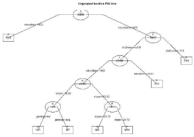
#we have a tree, but elevation as dominant variable. This doesn't
#sound realistic for the beetles distribution. For testing purpose we
#try again without elevation:
tree <- rpart(presence ~ .,data=mybugsites[,c(6:11)], cp=0.0)
tree
plot(tree,uniform=T,branch=.5, main="Unpruned beetles P/A tree II", cex=0.5)
text(tree,use.n=T,all=T,fancy=T)
#get suggestions where to prune the tree from plot 'cp' command:
plotcp(tree)
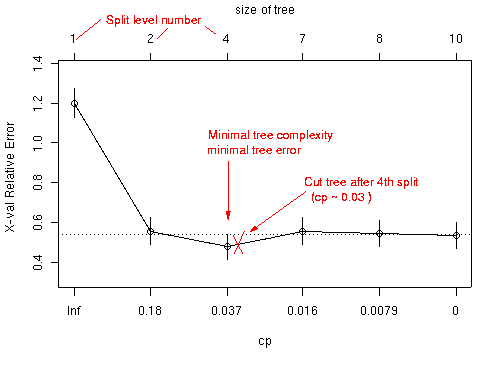
printcp(tree)
# 1-SE rule:
# min(xerror)+xstd of min(xerror)= threshold
# the BEST tree is the biggest tree with xerror less than threshold
#
## UNFINISHED - pruning needs discussion
## another problem is the proper selection of absence data.
#text tree:
#print(tree)
#printcp(tree)
#prune tree: TODO
#tree.p1 <- prune(tree,cp=0.025926)
#plot(tree.p1,uniform=T,branch=.5, main="Unpruned beetles P/A tree II", cex=0.5)
#text(tree.p1,use.n=T,all=T,fancy=T)
Predictive model: spatial predictions from the tree model
For now we use the unpruned tree to perform the spatial prediction.
The prediction requires to have the maps in R memory.
## initialize for output, all the region, including NA from GRASS
#load only used variables (see 'tree'):
#    Variables actually used in tree construction:
#    [1] aspect     dist2water geology    slope      vegetation
#To avoid problems we import also categorial data as numeric and reset
#later to factors:
mypred <- rast.get(G, c("aspect","dist2water.m","geology","slope","vegcover"),cat=(c(F,F,F,F,F)))
names(mypred) <- c("aspect","dist2water","geology","slope","vegetation")
str(mypred)

#make vegetation and geology factors:
mypred$vegetation <- as.factor(mypred$vegetation)
summary(mypred$vegetation)
mypred$geology    <- as.factor(mypred$geology)
str(mypred)
# ... should look like this:
#List of 5
# $ aspect    : num [1:294978] NA NA NA NA NA NA NA NA NA NA ...
# $ dist2water: num [1:294978] 210 210 210 210 210 240 240 270 270 300 ...
# $ geology   : Factor w/ 9 levels "1","2","3","4",..: NA NA NA NA NA NA NA NA NA NA ...
# $ slope     : num [1:294978] NA NA NA NA NA NA NA NA NA NA ...
# $ vegetation: Factor w/ 6 levels "1","2","3","4",..: 2 2 2 6 6 6 6 6 6 6 ...

#check names of vegetation and geology classes:
system("r.cats vegcover")
system("r.cats geology")
summary(mybugsites[,c(5,7:11)])

#preparation for prediction from model (using pruned tree):
# (rpart wants the data as data.frame)
mypredF <- as.data.frame(mypred)
summary(mypredF)

#predict (spatialization) using only active raster cells: We use na.omit()
#to eliminate all pixel rows with one or more NAs in the variable columns.
outmap   <- predict(tree,newdata=mypredF, type="class")

#An error message may appear like this:
#-> Error in model.frame.default(Terms, newdata, na.action = act, xlev =
#   attr(object,  :
#        factor geology has new level(s) 2
#==> this indicates that the sample data do not contain any occurency of
#    geology class 2. We either have to redo the "absence" random data,
#    or, we can remove 'geology class 2' from the mypredF data.frame:
#
#Well. We have to use a sort of trick to eliminate 'geology class 2'
#as it is a factor (as.numeric(as.character(factors) is needed to avoid
#that R picks the position of the level instead of the value!):
geologytmp<- as.numeric(as.character(mypredF$geology))
str(geologytmp)
summary(geologytmp==2)

#replace geology class 2 with NA:
geologytmp[geologytmp==2]<-NA
summary(geologytmp==2)
#-> the class 2 values should be NA now

#restore the updated geology variable in the data frame:
mypredF$geology<-as.factor(geologytmp)
summary(mypredF$geology)
rm(geologytmp)

#now we retry the tree:
outmap   <- predict(tree,newdata=mypredF, type="class")
summary(outmap)
# ... should print something like this:
#     A      P
#234320  60658

str(outmap)
# ... should print something like this:
# Factor w/ 2 levels "A","P": 1 1 1 1 1 1 1 1 1 1 ...
# - attr(*, "names")= chr [1:294978] "1" "2" "3" "4" ...

str(G$Ncells)
# ... should print something like this:
# int 294978
#
# The number identical to A/P values indicates that we have predicted for
# every raster cell as desired.

#create prob map:
outmap.p <- predict(tree,newdata=mypredF, type="prob")
summary(outmap.p)

#absence probability map:
plot(G, outmap.p[,1])
title("Absence probability map")
#presence probability map:
plot(G, outmap.p[,2])
title("Presence probability map")
Verification of the prediction quality: ROC plots
#get ROC library from http://www.bioconductor.org

library(ROC)

#trick to change P,A to 1,0:
truthvalues <- unclass(mybugsites$presence)
truthvalues2 <- as.numeric(truthvalues-1)
roc1 <- rocdemo.sca(truth=truthvalues2, data=outmap.p,
        rule=dxrule.sca, seqlen=5)
auc <- AUC(roc1)
print(auc)
plot(roc1, line=TRUE, show.thresh=TRUE, col="blue")
Writing the results back to GIS
#write out the result to GRASS:
rast.put(G, layer=outmap, lname="rpart.bugrisk")
rast.put(G, layer=outmap.p[,1], lname="rpart.bugrisk.probA")
rast.put(G, layer=outmap.p[,2], lname="rpart.bugrisk.probP")

#let's look at the result:
system("d.mon x0")
system("d.rast.leg rpart.bugrisk")

system("d.rast elevation.10m")
system("d.rast -o rpart.bugrisk cat=2")
system("d.vect mybugsites icon='basic/diamond' fcol=red")

system("r.colors rpart.bugrisk.probA col=ryg")
system("d.rast.leg rpart.bugrisk.probA")
system("echo Bugs absence probability | d.text")

system("r.colors rpart.bugrisk.probP col=ryg")
system("d.rast.leg rpart.bugrisk.probP")
system("echo Bugs presence probability | d.text")

#ciao:
q()

#look at the resulting GRASS map:
d.mon x0
d.rast.leg rpart.bugrisk
d.rast.leg rpart.bugrisk.probA
d.rast.leg rpart.bugrisk.probP

#That's it :-)
#TODO - Pruning the tree should be improved in this example.
© 2003-2006 Markus Neteler (neteler AT itc.it)
Back
Course HOME
Last change:
$Date: 2006-12-11 16:53:59 +0100 (Mon, 11 Dec 2006) $